#@title Importar librerías
#importar librerías necesarias
import os
import random
import numpy as np
import pandas as pd
from tqdm.notebook import tqdm
from matplotlib import pyplot as plt
import seaborn as sns

import tensorflow_datasets as tfds
import tensorflow as tfResolviendo diversidad de tareas con RNNs
Última actualización: 09/05/2025![]()
#@title Funciones complementarias

def plot_graphs(history, metric):
  plt.plot(history.history[metric])
  plt.plot(history.history['val_'+metric], '')
  plt.xlabel("Epochs")
  plt.ylabel(metric)
  plt.legend([metric, 'val_'+metric])

def plot_variables(df, date_time):
    plot_cols = ['T (degC)', 'p (mbar)', 'rho (g/m**3)']
    plot_features = df[plot_cols]
    plot_features.index = date_time
    _ = plot_features.plot(subplots=True)

    plot_features = df[plot_cols][:480]
    plot_features.index = date_time[:480]
    _ = plot_features.plot(subplots=True)

def read_dataset_clima():

    zip_path = tf.keras.utils.get_file(
        origin='https://storage.googleapis.com/tensorflow/tf-keras-datasets/jena_climate_2009_2016.csv.zip',
        fname='jena_climate_2009_2016.csv.zip',
        extract=True)
    csv_path, _ = os.path.splitext(zip_path)

    df = pd.read_csv(csv_path+'/'+'jena_climate_2009_2016.csv')
    # Slice [start:stop:step], starting from index 5 take every 6th record.
    df = df[5::6]

    date_time = pd.to_datetime(df.pop('Date Time'), format='%d.%m.%Y %H:%M:%S')

    return df, date_time

def split_data(df):
    column_indices = {name: i for i, name in enumerate(df.columns)}

    n = len(df)
    train_df = df[0:int(n*0.7)]
    val_df = df[int(n*0.7):int(n*0.9)]
    test_df = df[int(n*0.9):]

    num_features = df.shape[1]

    return train_df, val_df, test_df, num_features, column_indices

def normalizacion_datos(train_df, val_df, test_df):
    train_mean = train_df.mean()
    train_std = train_df.std()

    train_df = (train_df - train_mean) / train_std
    val_df = (val_df - train_mean) / train_std
    test_df = (test_df - train_mean) / train_std

    return train_df, val_df, test_df


class WindowGenerator():
  def __init__(self, input_width, label_width, shift,
               train_df, val_df, test_df,
               label_columns=None):
    # Store the raw data.
    self.train_df = train_df
    self.val_df = val_df
    self.test_df = test_df

    # Work out the label column indices.
    self.label_columns = label_columns
    if label_columns is not None:
      self.label_columns_indices = {name: i for i, name in
                                    enumerate(label_columns)}
    self.column_indices = {name: i for i, name in
                           enumerate(train_df.columns)}

    # Work out the window parameters.
    self.input_width = input_width
    self.label_width = label_width
    self.shift = shift

    self.total_window_size = input_width + shift

    self.input_slice = slice(0, input_width)
    self.input_indices = np.arange(self.total_window_size)[self.input_slice]

    self.label_start = self.total_window_size - self.label_width
    self.labels_slice = slice(self.label_start, None)
    self.label_indices = np.arange(self.total_window_size)[self.labels_slice]

  def __repr__(self):
    return '\n'.join([
        f'Total window size: {self.total_window_size}',
        f'Input indices: {self.input_indices}',
        f'Label indices: {self.label_indices}',
        f'Label column name(s): {self.label_columns}'])


def split_window(self, features):
  inputs = features[:, self.input_slice, :]
  labels = features[:, self.labels_slice, :]
  if self.label_columns is not None:
    labels = tf.stack(
        [labels[:, :, self.column_indices[name]] for name in self.label_columns],
        axis=-1)

  # Slicing doesn't preserve static shape information, so set the shapes
  # manually. This way the `tf.data.Datasets` are easier to inspect.
  inputs.set_shape([None, self.input_width, None])
  labels.set_shape([None, self.label_width, None])

  return inputs, labels

def plot(self, model=None, plot_col='T (degC)', max_subplots=3):
  inputs, labels = self.example
  plt.figure(figsize=(12, 8))
  plot_col_index = self.column_indices[plot_col]
  max_n = min(max_subplots, len(inputs))
  for n in range(max_n):
    plt.subplot(max_n, 1, n+1)
    plt.ylabel(f'{plot_col} [normed]')
    plt.plot(self.input_indices, inputs[n, :, plot_col_index],
             label='Inputs', marker='.', zorder=-10)

    if self.label_columns:
      label_col_index = self.label_columns_indices.get(plot_col, None)
    else:
      label_col_index = plot_col_index

    if label_col_index is None:
      continue

    plt.scatter(self.label_indices, labels[n, :, label_col_index],
                edgecolors='k', label='Labels', c='#2ca02c', s=64)
    if model is not None:
      predictions = model(inputs)
      plt.scatter(self.label_indices, predictions[n, :, label_col_index],
                  marker='X', edgecolors='k', label='Predictions',
                  c='#ff7f0e', s=64)

    if n == 0:
      plt.legend()

  plt.xlabel('Time [h]')

def make_dataset(self, data):
  data = np.array(data, dtype=np.float32)
  ds = tf.keras.utils.timeseries_dataset_from_array(
      data=data,
      targets=None,
      sequence_length=self.total_window_size,
      sequence_stride=1,
      shuffle=True,
      batch_size=32,)

  ds = ds.map(self.split_window)

  return ds


@property
def train(self):
  return self.make_dataset(self.train_df)

@property
def val(self):
  return self.make_dataset(self.val_df)

@property
def test(self):
  return self.make_dataset(self.test_df)

@property
def example(self):
  """Get and cache an example batch of `inputs, labels` for plotting."""
  result = getattr(self, '_example', None)
  if result is None:
    # No example batch was found, so get one from the `.train` dataset
    result = next(iter(self.train))
    # And cache it for next time
    self._example = result
  return result


WindowGenerator.plot = plot
WindowGenerator.split_window = split_window
WindowGenerator.make_dataset = make_dataset
WindowGenerator.train = train
WindowGenerator.val = val
WindowGenerator.test = test
WindowGenerator.example = example
Escenarios de uso de las redes neuronales recurrentes.

Clasificación de texto usando RNNs (Relación muchas entradas a una salida)
En este escenario se reciben multiples entradas pero solo se genera una salida. Aquí podemos abordar el ejemplo más común que es la clasificación de texto.
Descargar el dataset de reviews de peliculas usando Tensorflow.
El gran conjunto de datos de críticas de películas de IMDB es un conjunto de datos de clasificación binaria: todas las críticas tienen un sentimiento positivo o negativo.
dataset, info = tfds.load('imdb_reviews', with_info=True,
                          as_supervised=True)
train_dataset, test_dataset = dataset['train'], dataset['test']
WARNING:absl:Variant folder /root/tensorflow_datasets/imdb_reviews/plain_text/1.0.0 has no dataset_info.jsonDownloading and preparing dataset Unknown size (download: Unknown size, generated: Unknown size, total: Unknown size) to /root/tensorflow_datasets/imdb_reviews/plain_text/1.0.0...Dataset imdb_reviews downloaded and prepared to /root/tensorflow_datasets/imdb_reviews/plain_text/1.0.0. Subsequent calls will reuse this data.# contar cuantas muestras tiene train_dataset y test_dataset
print(info.splits){Split('train'): <SplitInfo num_examples=25000, num_shards=1>, Split('test'): <SplitInfo num_examples=25000, num_shards=1>, Split('unsupervised'): <SplitInfo num_examples=50000, num_shards=1>}# extraer una muestra del conjunto de entrenamiento
train_example, train_label = next(iter(train_dataset.batch(1)))
print('Para la etiqueta: {} se tiene el texto: {}'.format(train_label, train_example.numpy()))Para la etiqueta: [0] se tiene el texto: [b"This was an absolutely terrible movie. Don't be lured in by Christopher Walken or Michael Ironside. Both are great actors, but this must simply be their worst role in history. Even their great acting could not redeem this movie's ridiculous storyline. This movie is an early nineties US propaganda piece. The most pathetic scenes were those when the Columbian rebels were making their cases for revolutions. Maria Conchita Alonso appeared phony, and her pseudo-love affair with Walken was nothing but a pathetic emotional plug in a movie that was devoid of any real meaning. I am disappointed that there are movies like this, ruining actor's like Christopher Walken's good name. I could barely sit through it."]Las siguientes lineas son para optimizar los conjuntos y que el entrenamiento sea más acelerado.
BUFFER_SIZE = 10000
BATCH_SIZE = 32

# optimización para train
train_dataset = train_dataset.shuffle(BUFFER_SIZE).batch(BATCH_SIZE).prefetch(tf.data.AUTOTUNE)

# optimización para test
test_dataset = test_dataset.batch(BATCH_SIZE).prefetch(tf.data.AUTOTUNE)
# muestras para el conjunto de test
for ejemplo, label in test_dataset.take(1):
print('textos: ', ejemplo.numpy()[:3])
print()
print('labels: ', label.numpy()[:3])textos: [b"There are films that make careers. For George Romero, it was NIGHT OF THE LIVING DEAD; for Kevin Smith, CLERKS; for Robert Rodriguez, EL MARIACHI. Add to that list Onur Tukel's absolutely amazing DING-A-LING-LESS. Flawless film-making, and as assured and as professional as any of the aforementioned movies. I haven't laughed this hard since I saw THE FULL MONTY. (And, even then, I don't think I laughed quite this hard... So to speak.) Tukel's talent is considerable: DING-A-LING-LESS is so chock full of double entendres that one would have to sit down with a copy of this script and do a line-by-line examination of it to fully appreciate the, uh, breadth and width of it. Every shot is beautifully composed (a clear sign of a sure-handed director), and the performances all around are solid (there's none of the over-the-top scenery chewing one might've expected from a film like this). DING-A-LING-LESS is a film whose time has come."
b"A blackly comic tale of a down-trodden priest, Nazarin showcases the economy that Luis Bunuel was able to achieve in being able to tell a deeply humanist fable with a minimum of fuss. As an output from his Mexican era of film making, it was an invaluable talent to possess, with little money and extremely tight schedules. Nazarin, however, surpasses many of Bunuel's previous Mexican films in terms of the acting (Francisco Rabal is excellent), narrative and theme.<br /><br />The theme, interestingly, is something that was explored again in Viridiana, made three years later in Spain. It concerns the individual's struggle for humanity and altruism amongst a society that rejects any notion of virtue. Father Nazarin, however, is portrayed more sympathetically than Sister Viridiana. Whereas the latter seems to choose charity because she wishes to atone for her (perceived) sins, Nazarin's whole existence and reason for being seems to be to help others, whether they (or we) like it or not. The film's last scenes, in which he casts doubt on his behaviour and, in a split second, has to choose between the life he has been leading or the conventional life that is expected of a priest, are so emotional because they concern his moral integrity and we are never quite sure whether it remains intact or not.<br /><br />This is a remarkable film and I would urge anyone interested in classic cinema to seek it out. It is one of Bunuel's most moving films, and encapsulates many of his obsessions: frustrated desire, mad love, religious hypocrisy etc. In my view 'Nazarin' is second only to 'The Exterminating Angel', in terms of his Mexican movies, and is certainly near the top of the list of Bunuel's total filmic output."
b'Scary Movie 1-4, Epic Movie, Date Movie, Meet the Spartans, Not another Teen Movie and Another Gay Movie. Making "Superhero Movie" the eleventh in a series that single handily ruined the parody genre. Now I\'ll admit it I have a soft spot for classics such as Airplane and The Naked Gun but you know you\'ve milked a franchise so bad when you can see the gags a mile off. In fact the only thing that might really temp you into going to see this disaster is the incredibly funny but massive sell-out Leslie Neilson.<br /><br />You can tell he needs the money, wither that or he intends to go down with the ship like a good Capitan would. In no way is he bringing down this genre but hell he\'s not helping it. But if I feel sorry for anybody in this film its decent actor Drake Bell who is put through an immense amount of embarrassment. The people who are put through the largest amount of torture by far however is the audience forced to sit through 90 minutes of laughless bile no funnier than herpes.<br /><br />After spoofing disaster films in Airplane!, police shows in The Naked Gun, and Hollywood horrors in Scary Movie 3 and 4, producer David Zucker sets his satirical sights on the superhero genre with this anarchic comedy lampooning everything from Spider-Man to X-Men and Superman Returns.<br /><br />Shortly after being bitten by a genetically altered dragonfly, high-school outcast Rick Riker (Drake Bell) begins to experience a startling transformation. Now Rick\'s skin is as strong as steel, and he possesses the strength of ten men. Determined to use his newfound powers to fight crime, Rick creates a special costume and assumes the identity of The Dragonfly -- a fearless crime fighter dedicated to keeping the streets safe for law-abiding citizens.<br /><br />But every superhero needs a nemesis, and after Lou Landers (Christopher McDonald) is caught in the middle of an experiment gone horribly awry, he develops the power to leech the life force out of anyone he meets and becomes the villainous Hourglass. Intent on achieving immortality, the Hourglass attempts to gather as much life force as possible as the noble Dragonfly sets out to take down his archenemy and realize his destiny as a true hero. Craig Mazin writes and directs this low-flying spoof.<br /><br />featuring Tracy Morgan, Pamela Anderson, Leslie Nielsen, Marion Ross, Jeffrey Tambor, and Regina Hall.<br /><br />Hell Superhero Movie may earn some merit in the fact that it\'s a hell of a lot better than Meet the Spartans and Epic Movie. But with great responsibility comes one of the worst outings of 2008 to date. Laughless but a little less irritating than Meet the Spartans. And in the same sense much more forgettable than meet the Spartans. But maybe that\'s a good reason. There are still some of us trying to scrape away the stain that was Meet the Spartans from our memory.<br /><br />My final verdict? Avoid, unless you\'re one of thoses people who enjoy such car crash cinema. As bad as Date Movie and Scary Movie 2 but not quite as bad as Meet the Spartans or Epic Movie. Super Villain.']
labels: [1 1 0]Pre-procesamiento y modelado.

Explicación del modelo:
Este modelo se puede construir como un tf.keras.Sequential.
La primera capa (amarilla) es el codificador, que convierte el texto en una secuencia de índices de tokens.
Después del codificador hay una capa de embedding (verde). Una capa de embedding almacena un vector por palabra. Cuando se llama, convierte las secuencias de índices de palabras en secuencias de vectores. Estos vectores son entrenables. Después del entrenamiento (con suficientes datos), las palabras con significados similares a menudo tienen vectores similares.
Una red neuronal recurrente (RNN) procesa la entrada secuencial iterando a través de los elementos. Las RNN pasan las salidas de un instante de tiempo a su entrada en el siguiente instante de tiempo.
La capa tf.keras.layers.Bidirectional también se puede usar con una capa RNN. Esto propaga la entrada hacia adelante y hacia atrás a través de la capa RNN y luego concatena la salida final.
La principal ventaja de una RNN bidireccional es que la señal desde el comienzo de la entrada no necesita ser procesada a lo largo de cada instante de tiempo para afectar la salida.
La principal desventaja de una RNN bidireccional es que no se pueden transmitir predicciones de manera eficiente a medida que se agregan palabras al final.
Después de que la RNN ha convertido la secuencia en un solo vector, las dos capas Dense realizan un procesamiento final y convierten esta representación vectorial en un solo valor como salida de clasificación.
Capa Codificador (Text Vectorization)
El texto sin procesar cargado por tfds necesita ser procesado antes de que pueda ser utilizado en un modelo. La forma más sencilla de procesar texto para el entrenamiento es utilizando la capa TextVectorization.
Explicación:
La capa TextVectorization es una herramienta en TensorFlow que transforma texto sin procesar en una representación numérica que los modelos de aprendizaje automático pueden entender. Convierte las palabras en vectores, lo que facilita el entrenamiento del modelo. Esto incluye tareas como:
- Tokenización: Dividir el texto en palabras o subpalabras.
- Normalización: Convertir todo el texto a minúsculas, eliminar caracteres especiales, etc.
- Vectorización: Asignar un índice o valor numérico a cada palabra o token, lo que permite representarlo como una matriz numérica.
VOCAB_SIZE = 1000
encoder = tf.keras.layers.TextVectorization(
    max_tokens=VOCAB_SIZE)

# Crea la capa y pasa el texto del conjunto de datos al método .adapt de la capa
encoder.adapt(train_dataset.map(lambda text, label: text))
El método .adapt se utiliza para “entrenar” la capa en el conjunto de datos de texto. Esto significa que la capa analizará el texto y aprenderá el vocabulario, así como otras características (como la frecuencia de las palabras) que serán útiles para la vectorización
# revisar los primeros 20 elementos del vocabulario creado
vocab = np.array(encoder.get_vocabulary())
vocab[:20]
array(['', '[UNK]', 'the', 'and', 'a', 'of', 'to', 'is', 'in', 'it', 'i',
'this', 'that', 'br', 'was', 'as', 'for', 'with', 'movie', 'but'],
dtype='<U14')Una vez que el vocabulario está establecido, la capa puede codificar el texto en índices. Los tensores de índices se rellenan con ceros hasta la secuencia más larga en el batch (a menos que establezcas una longitud de salida fija).
encoded_ejemplo = encoder(ejemplo)[:3].numpy()
encoded_ejemplo
array([[ 48, 24, 95, ..., 0, 0, 0],
[ 4, 1, 723, ..., 0, 0, 0],
[633, 18, 1, ..., 18, 1, 1]])# Visualizamos algunas oraciones
for n in range(3):
print("Original: ", ejemplo[n].numpy())
# intentar decodificar solo usando el vocab
print("Round-trip: ", " ".join(vocab[encoded_ejemplo[n]]))
print()Original: b"There are films that make careers. For George Romero, it was NIGHT OF THE LIVING DEAD; for Kevin Smith, CLERKS; for Robert Rodriguez, EL MARIACHI. Add to that list Onur Tukel's absolutely amazing DING-A-LING-LESS. Flawless film-making, and as assured and as professional as any of the aforementioned movies. I haven't laughed this hard since I saw THE FULL MONTY. (And, even then, I don't think I laughed quite this hard... So to speak.) Tukel's talent is considerable: DING-A-LING-LESS is so chock full of double entendres that one would have to sit down with a copy of this script and do a line-by-line examination of it to fully appreciate the, uh, breadth and width of it. Every shot is beautifully composed (a clear sign of a sure-handed director), and the performances all around are solid (there's none of the over-the-top scenery chewing one might've expected from a film like this). DING-A-LING-LESS is a film whose time has come."
Round-trip: there are films that make [UNK] for george [UNK] it was night of the living dead for [UNK] [UNK] [UNK] for robert [UNK] [UNK] [UNK] add to that [UNK] [UNK] [UNK] absolutely amazing [UNK] [UNK] [UNK] and as [UNK] and as [UNK] as any of the [UNK] movies i havent [UNK] this hard since i saw the full [UNK] and even then i dont think i [UNK] quite this hard so to [UNK] [UNK] talent is [UNK] [UNK] is so [UNK] full of [UNK] [UNK] that one would have to sit down with a [UNK] of this script and do a [UNK] [UNK] of it to [UNK] [UNK] the [UNK] [UNK] and [UNK] of it every shot is [UNK] [UNK] a clear [UNK] of a [UNK] director and the performances all around are [UNK] theres none of the [UNK] [UNK] [UNK] one [UNK] expected from a film like this [UNK] is a film whose time has come
Original: b"A blackly comic tale of a down-trodden priest, Nazarin showcases the economy that Luis Bunuel was able to achieve in being able to tell a deeply humanist fable with a minimum of fuss. As an output from his Mexican era of film making, it was an invaluable talent to possess, with little money and extremely tight schedules. Nazarin, however, surpasses many of Bunuel's previous Mexican films in terms of the acting (Francisco Rabal is excellent), narrative and theme.<br /><br />The theme, interestingly, is something that was explored again in Viridiana, made three years later in Spain. It concerns the individual's struggle for humanity and altruism amongst a society that rejects any notion of virtue. Father Nazarin, however, is portrayed more sympathetically than Sister Viridiana. Whereas the latter seems to choose charity because she wishes to atone for her (perceived) sins, Nazarin's whole existence and reason for being seems to be to help others, whether they (or we) like it or not. The film's last scenes, in which he casts doubt on his behaviour and, in a split second, has to choose between the life he has been leading or the conventional life that is expected of a priest, are so emotional because they concern his moral integrity and we are never quite sure whether it remains intact or not.<br /><br />This is a remarkable film and I would urge anyone interested in classic cinema to seek it out. It is one of Bunuel's most moving films, and encapsulates many of his obsessions: frustrated desire, mad love, religious hypocrisy etc. In my view 'Nazarin' is second only to 'The Exterminating Angel', in terms of his Mexican movies, and is certainly near the top of the list of Bunuel's total filmic output."
Round-trip: a [UNK] comic tale of a [UNK] [UNK] [UNK] [UNK] the [UNK] that [UNK] [UNK] was able to [UNK] in being able to tell a [UNK] [UNK] [UNK] with a [UNK] of [UNK] as an [UNK] from his [UNK] [UNK] of film making it was an [UNK] talent to [UNK] with little money and extremely [UNK] [UNK] [UNK] however [UNK] many of [UNK] previous [UNK] films in [UNK] of the acting [UNK] [UNK] is excellent [UNK] and [UNK] br the theme [UNK] is something that was [UNK] again in [UNK] made three years later in [UNK] it [UNK] the [UNK] [UNK] for [UNK] and [UNK] [UNK] a society that [UNK] any [UNK] of [UNK] father [UNK] however is portrayed more [UNK] than sister [UNK] [UNK] the [UNK] seems to [UNK] [UNK] because she [UNK] to [UNK] for her [UNK] [UNK] [UNK] whole [UNK] and reason for being seems to be to help others whether they or we like it or not the films last scenes in which he [UNK] doubt on his [UNK] and in a [UNK] second has to [UNK] between the life he has been leading or the [UNK] life that is expected of a [UNK] are so emotional because they [UNK] his [UNK] [UNK] and we are never quite sure whether it [UNK] [UNK] or [UNK] br this is a [UNK] film and i would [UNK] anyone interested in classic cinema to [UNK] it out it is one of [UNK] most moving films and [UNK] many of his [UNK] [UNK] [UNK] [UNK] love [UNK] [UNK] etc in my view [UNK] is second only to the [UNK] [UNK] in [UNK] of his [UNK] movies and is certainly near the top of the [UNK] of [UNK] total [UNK] [UNK]
Original: b'Scary Movie 1-4, Epic Movie, Date Movie, Meet the Spartans, Not another Teen Movie and Another Gay Movie. Making "Superhero Movie" the eleventh in a series that single handily ruined the parody genre. Now I\'ll admit it I have a soft spot for classics such as Airplane and The Naked Gun but you know you\'ve milked a franchise so bad when you can see the gags a mile off. In fact the only thing that might really temp you into going to see this disaster is the incredibly funny but massive sell-out Leslie Neilson.<br /><br />You can tell he needs the money, wither that or he intends to go down with the ship like a good Capitan would. In no way is he bringing down this genre but hell he\'s not helping it. But if I feel sorry for anybody in this film its decent actor Drake Bell who is put through an immense amount of embarrassment. The people who are put through the largest amount of torture by far however is the audience forced to sit through 90 minutes of laughless bile no funnier than herpes.<br /><br />After spoofing disaster films in Airplane!, police shows in The Naked Gun, and Hollywood horrors in Scary Movie 3 and 4, producer David Zucker sets his satirical sights on the superhero genre with this anarchic comedy lampooning everything from Spider-Man to X-Men and Superman Returns.<br /><br />Shortly after being bitten by a genetically altered dragonfly, high-school outcast Rick Riker (Drake Bell) begins to experience a startling transformation. Now Rick\'s skin is as strong as steel, and he possesses the strength of ten men. Determined to use his newfound powers to fight crime, Rick creates a special costume and assumes the identity of The Dragonfly -- a fearless crime fighter dedicated to keeping the streets safe for law-abiding citizens.<br /><br />But every superhero needs a nemesis, and after Lou Landers (Christopher McDonald) is caught in the middle of an experiment gone horribly awry, he develops the power to leech the life force out of anyone he meets and becomes the villainous Hourglass. Intent on achieving immortality, the Hourglass attempts to gather as much life force as possible as the noble Dragonfly sets out to take down his archenemy and realize his destiny as a true hero. Craig Mazin writes and directs this low-flying spoof.<br /><br />featuring Tracy Morgan, Pamela Anderson, Leslie Nielsen, Marion Ross, Jeffrey Tambor, and Regina Hall.<br /><br />Hell Superhero Movie may earn some merit in the fact that it\'s a hell of a lot better than Meet the Spartans and Epic Movie. But with great responsibility comes one of the worst outings of 2008 to date. Laughless but a little less irritating than Meet the Spartans. And in the same sense much more forgettable than meet the Spartans. But maybe that\'s a good reason. There are still some of us trying to scrape away the stain that was Meet the Spartans from our memory.<br /><br />My final verdict? Avoid, unless you\'re one of thoses people who enjoy such car crash cinema. As bad as Date Movie and Scary Movie 2 but not quite as bad as Meet the Spartans or Epic Movie. Super Villain.'
Round-trip: scary movie [UNK] [UNK] movie [UNK] movie meet the [UNK] not another [UNK] movie and another [UNK] movie making [UNK] movie the [UNK] in a series that single [UNK] [UNK] the [UNK] genre now ill admit it i have a [UNK] [UNK] for [UNK] such as [UNK] and the [UNK] [UNK] but you know youve [UNK] a [UNK] so bad when you can see the [UNK] a [UNK] off in fact the only thing that might really [UNK] you into going to see this [UNK] is the incredibly funny but [UNK] [UNK] [UNK] [UNK] br you can tell he needs the money [UNK] that or he [UNK] to go down with the [UNK] like a good [UNK] would in no way is he [UNK] down this genre but hell hes not [UNK] it but if i feel sorry for [UNK] in this film its decent actor [UNK] [UNK] who is put through an [UNK] [UNK] of [UNK] the people who are put through the [UNK] [UNK] of [UNK] by far however is the audience forced to sit through [UNK] minutes of [UNK] [UNK] no [UNK] than [UNK] br after [UNK] [UNK] films in [UNK] police shows in the [UNK] [UNK] and hollywood [UNK] in scary movie 3 and 4 [UNK] david [UNK] sets his [UNK] [UNK] on the [UNK] genre with this [UNK] comedy [UNK] everything from [UNK] to [UNK] and [UNK] [UNK] br [UNK] after being [UNK] by a [UNK] [UNK] [UNK] [UNK] [UNK] [UNK] [UNK] [UNK] [UNK] begins to experience a [UNK] [UNK] now [UNK] [UNK] is as strong as [UNK] and he [UNK] the [UNK] of ten men [UNK] to use his [UNK] [UNK] to fight crime [UNK] [UNK] a special [UNK] and [UNK] the [UNK] of the [UNK] a [UNK] crime [UNK] [UNK] to [UNK] the [UNK] [UNK] for [UNK] [UNK] br but every [UNK] needs a [UNK] and after [UNK] [UNK] [UNK] [UNK] is [UNK] in the middle of an [UNK] gone [UNK] [UNK] he [UNK] the power to [UNK] the life [UNK] out of anyone he meets and becomes the [UNK] [UNK] [UNK] on [UNK] [UNK] the [UNK] attempts to [UNK] as much life [UNK] as possible as the [UNK] [UNK] sets out to take down his [UNK] and realize his [UNK] as a true hero [UNK] [UNK] [UNK] and [UNK] this [UNK] [UNK] br [UNK] [UNK] [UNK] [UNK] [UNK] [UNK] [UNK] [UNK] [UNK] [UNK] [UNK] and [UNK] [UNK] br hell [UNK] movie may [UNK] some [UNK] in the fact that its a hell of a lot better than meet the [UNK] and [UNK] movie but with great [UNK] comes one of the worst [UNK] of [UNK] to [UNK] [UNK] but a little less [UNK] than meet the [UNK] and in the same sense much more [UNK] than meet the [UNK] but maybe thats a good reason there are still some of us trying to [UNK] away the [UNK] that was meet the [UNK] from our [UNK] br my final [UNK] avoid unless youre one of [UNK] people who enjoy such car [UNK] cinema as bad as [UNK] movie and scary movie 2 but not quite as bad as meet the [UNK] or [UNK] movie [UNK] [UNK]
Creación del modelo usando keras
'''model = tf.keras.Sequential([
    encoder,
    tf.keras.layers.Embedding(
        input_dim=len(encoder.get_vocabulary()),
        output_dim=64,
        # Se ignora los valores en 0
        mask_zero=True),
    tf.keras.layers.Bidirectional(tf.keras.layers.LSTM(64), merge_mode='concat'),
    tf.keras.layers.Dense(64, activation='relu'),
    tf.keras.layers.Dense(1)
])'''

def rnn():
    # Ahora utilizamos la API funcional de Keras
    inputs = tf.keras.layers.Input(shape=(1,), dtype=tf.string)  # El input será una cadena de texto
    x = encoder(inputs)  # Aplicamos el encoder

    x = tf.keras.layers.Embedding(input_dim=len(encoder.get_vocabulary()), output_dim=64, mask_zero=True)(x)  # Capa de Embedding

    x = tf.keras.layers.Bidirectional(tf.keras.layers.LSTM(64, return_sequences=False), merge_mode='concat')(x)  # Capa LSTM Bidireccional

    x = tf.keras.layers.Dense(64, activation='relu')(x)  # Capa densa
    outputs = tf.keras.layers.Dense(1, activation='sigmoid')(x)  # Capa de salida

    # Definimos el modelo
    model = tf.keras.Model(inputs, outputs)

    return model

# crear la red RNN
model = rnn()

# Compilamos el modelo
model.compile(loss=tf.keras.losses.BinaryCrossentropy(from_logits=False),
              optimizer=tf.keras.optimizers.Adam(1e-4),
              metrics=['accuracy'])

# Verificamos la estructura del modelo
model.summary()
Model: "functional_1"
┏━━━━━━━━━━━━━━━━━━━━━┳━━━━━━━━━━━━━━━━━━━┳━━━━━━━━━━━━┳━━━━━━━━━━━━━━━━━━━┓
┃ Layer (type)        ┃ Output Shape      ┃    Param # ┃ Connected to      ┃
┡━━━━━━━━━━━━━━━━━━━━━╇━━━━━━━━━━━━━━━━━━━╇━━━━━━━━━━━━╇━━━━━━━━━━━━━━━━━━━┩
│ input_layer_1       │ (None, 1)         │          0 │ -                 │
│ (InputLayer)        │                   │            │                   │
├─────────────────────┼───────────────────┼────────────┼───────────────────┤
│ text_vectorization  │ (None, None)      │          0 │ input_layer_1[0]… │
│ (TextVectorization) │                   │            │                   │
├─────────────────────┼───────────────────┼────────────┼───────────────────┤
│ embedding_1         │ (None, None, 64)  │     64,000 │ text_vectorizati… │
│ (Embedding)         │                   │            │                   │
├─────────────────────┼───────────────────┼────────────┼───────────────────┤
│ not_equal_1         │ (None, None)      │          0 │ text_vectorizati… │
│ (NotEqual)          │                   │            │                   │
├─────────────────────┼───────────────────┼────────────┼───────────────────┤
│ bidirectional_1     │ (None, 128)       │     66,048 │ embedding_1[0][0… │
│ (Bidirectional)     │                   │            │ not_equal_1[0][0] │
├─────────────────────┼───────────────────┼────────────┼───────────────────┤
│ dense_2 (Dense)     │ (None, 64)        │      8,256 │ bidirectional_1[… │
├─────────────────────┼───────────────────┼────────────┼───────────────────┤
│ dense_3 (Dense)     │ (None, 1)         │         65 │ dense_2[0][0]     │
└─────────────────────┴───────────────────┴────────────┴───────────────────┘
Total params: 138,369 (540.50 KB)
Trainable params: 138,369 (540.50 KB)
Non-trainable params: 0 (0.00 B)
tf.keras.utils.plot_model(model, show_shapes=True, show_layer_names=True)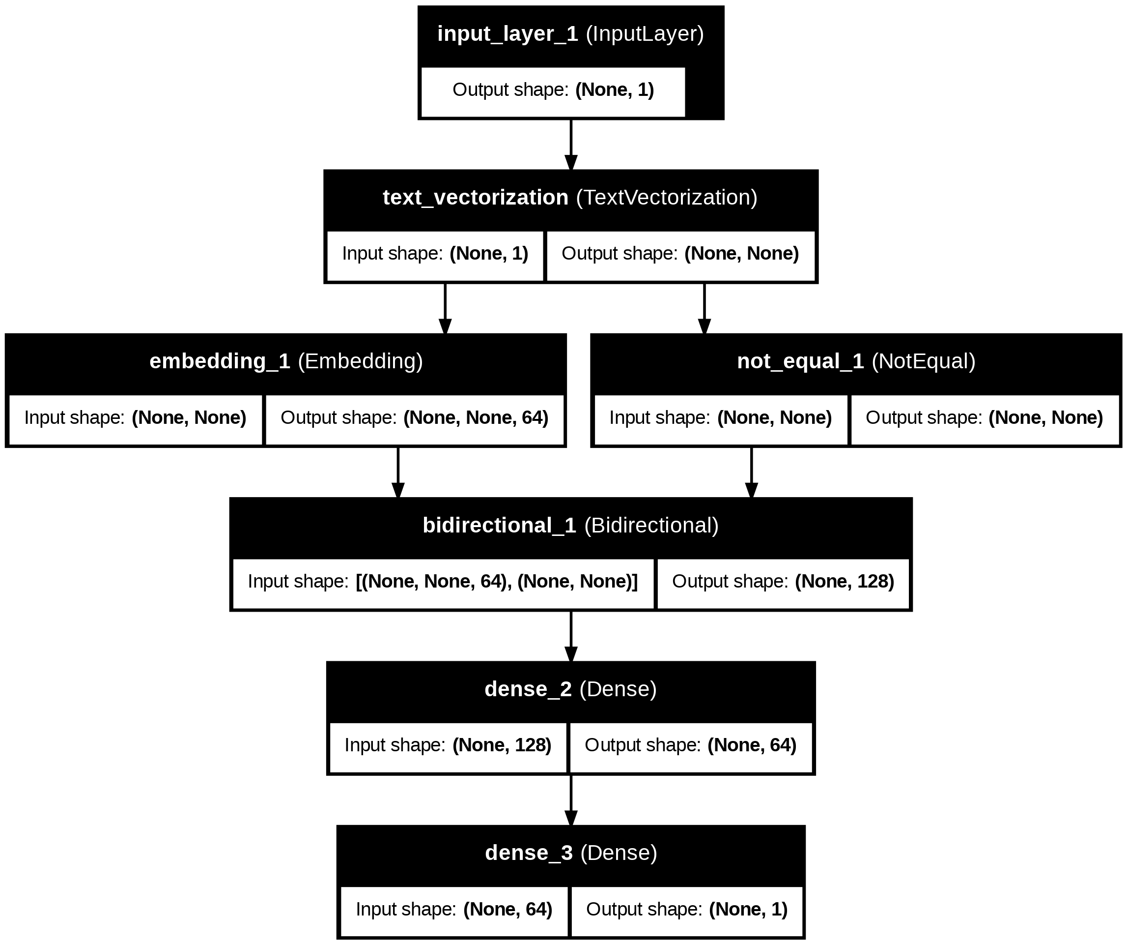
# El texto crudo que quieres predecir
sample_text = ('The movie was cool. The animation and the graphics were out of this world.')

# No es necesario hacer la vectorización manual aquí, simplemente pasa el texto crudo al modelo
predictions = model.predict(tf.constant([sample_text]))

# Imprime la predicción .. que debe ser casi 0.5 (neutralidad)
print(predictions[0])
1/1 ━━━━━━━━━━━━━━━━━━━━ 1s 1s/step [0.4999323]
Entrenamiento y evaluación del modelo
history = model.fit(train_dataset, epochs=10,
                    validation_data=test_dataset,
                    validation_steps=30)
Epoch 1/10 782/782 ━━━━━━━━━━━━━━━━━━━━ 39s 44ms/step - accuracy: 0.5798 - loss: 0.6706 - val_accuracy: 0.7823 - val_loss: 0.5019 Epoch 2/10 782/782 ━━━━━━━━━━━━━━━━━━━━ 40s 45ms/step - accuracy: 0.7957 - loss: 0.4493 - val_accuracy: 0.8271 - val_loss: 0.4129 Epoch 3/10 782/782 ━━━━━━━━━━━━━━━━━━━━ 41s 52ms/step - accuracy: 0.8513 - loss: 0.3502 - val_accuracy: 0.8427 - val_loss: 0.3751 Epoch 4/10 782/782 ━━━━━━━━━━━━━━━━━━━━ 82s 52ms/step - accuracy: 0.8605 - loss: 0.3311 - val_accuracy: 0.8521 - val_loss: 0.3591 Epoch 5/10 782/782 ━━━━━━━━━━━━━━━━━━━━ 74s 43ms/step - accuracy: 0.8665 - loss: 0.3233 - val_accuracy: 0.8698 - val_loss: 0.3445 Epoch 6/10 782/782 ━━━━━━━━━━━━━━━━━━━━ 36s 46ms/step - accuracy: 0.8688 - loss: 0.3157 - val_accuracy: 0.8687 - val_loss: 0.3407 Epoch 7/10 782/782 ━━━━━━━━━━━━━━━━━━━━ 82s 99ms/step - accuracy: 0.8722 - loss: 0.3120 - val_accuracy: 0.8531 - val_loss: 0.3814 Epoch 8/10 782/782 ━━━━━━━━━━━━━━━━━━━━ 41s 46ms/step - accuracy: 0.8702 - loss: 0.3176 - val_accuracy: 0.8490 - val_loss: 0.3559 Epoch 9/10 782/782 ━━━━━━━━━━━━━━━━━━━━ 41s 52ms/step - accuracy: 0.8701 - loss: 0.3108 - val_accuracy: 0.8646 - val_loss: 0.3362 Epoch 10/10 782/782 ━━━━━━━━━━━━━━━━━━━━ 75s 44ms/step - accuracy: 0.8703 - loss: 0.3075 - val_accuracy: 0.8302 - val_loss: 0.3808
test_loss, test_acc = model.evaluate(test_dataset)

print('Test Loss:', test_loss)
print('Test Accuracy:', test_acc)
782/782 ━━━━━━━━━━━━━━━━━━━━ 17s 22ms/step - accuracy: 0.8340 - loss: 0.3708 Test Loss: 0.37266772985458374 Test Accuracy: 0.8334000110626221
plt.figure(figsize=(12, 6))
plt.subplot(1, 2, 1)
plot_graphs(history, 'accuracy')
plt.ylim(None, 1)
plt.subplot(1, 2, 2)
plot_graphs(history, 'loss')
plt.ylim(0, None)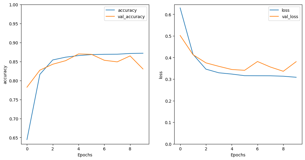
# realizar una predicción des pues de entrenar
sample_text = ('The movie was cool. The animation and the graphics were out of this world.')
predictions = model.predict(tf.constant([sample_text]))
print(predictions)
1/1 ━━━━━━━━━━━━━━━━━━━━ 0s 30ms/step [[0.6709632]]
# realizar una predicción des pues de entrenar
sample_text = ('The movie was very cool. The animation and the graphics were out of this world.')
predictions = model.predict(tf.constant([sample_text]))
print(predictions)
1/1 ━━━━━━━━━━━━━━━━━━━━ 0s 34ms/step [[0.71158457]]
Cómo podríamos agregar más capas LSTM para aumentar la complejidad del modelo?

Las capas recurrentes de Keras tienen dos modos disponibles que son controlados por el argumento del constructor return_sequences:
Si es False devuelve sólo la última salida para cada secuencia de entrada (un tensor 2D de forma (batch_size, output_features)). Este es el valor por defecto, utilizado en el modelo anterior.
Si es True se devuelven las secuencias completas de salidas sucesivas para cada paso de tiempo (un tensor 3D de forma (batch_size, timesteps, output_features)).
# model = tf.keras.Sequential([
    encoder,
    tf.keras.layers.Embedding(len(encoder.get_vocabulary()), 64, mask_zero=True),
    tf.keras.layers.Bidirectional(tf.keras.layers.LSTM(64,  return_sequences=True)),
    tf.keras.layers.Bidirectional(tf.keras.layers.LSTM(32)),
    tf.keras.layers.Dense(64, activation='relu'),
    tf.keras.layers.Dropout(0.5),
    tf.keras.layers.Dense(1)
])
Una o múltiples predicciones en el futuro usando LSTM con múltiples entradas.
En este ejercicio vamos a trabajar con series temporales. El objetivo es recibir múltiples entradas (ejemplo últimas 24 mediciones de temperatura a nivel de hora) y producir ya sea una o múltiples predicciones en el futuro. Para lograr esto, lo más importante es las ventanas de datos con los que se entrenan las redes recurrentes.

Leer datos
df, date_time = read_dataset_clima()df| p (mbar) | T (degC) | Tpot (K) | Tdew (degC) | rh (%) | VPmax (mbar) | VPact (mbar) | VPdef (mbar) | sh (g/kg) | H2OC (mmol/mol) | rho (g/m**3) | wv (m/s) | max. wv (m/s) | wd (deg) | |
|---|---|---|---|---|---|---|---|---|---|---|---|---|---|---|
| 5 | 996.50 | -8.05 | 265.38 | -8.78 | 94.40 | 3.33 | 3.14 | 0.19 | 1.96 | 3.15 | 1307.86 | 0.21 | 0.63 | 192.7 |
| 11 | 996.62 | -8.88 | 264.54 | -9.77 | 93.20 | 3.12 | 2.90 | 0.21 | 1.81 | 2.91 | 1312.25 | 0.25 | 0.63 | 190.3 |
| 17 | 996.84 | -8.81 | 264.59 | -9.66 | 93.50 | 3.13 | 2.93 | 0.20 | 1.83 | 2.94 | 1312.18 | 0.18 | 0.63 | 167.2 |
| 23 | 996.99 | -9.05 | 264.34 | -10.02 | 92.60 | 3.07 | 2.85 | 0.23 | 1.78 | 2.85 | 1313.61 | 0.10 | 0.38 | 240.0 |
| 29 | 997.46 | -9.63 | 263.72 | -10.65 | 92.20 | 2.94 | 2.71 | 0.23 | 1.69 | 2.71 | 1317.19 | 0.40 | 0.88 | 157.0 |
| ... | ... | ... | ... | ... | ... | ... | ... | ... | ... | ... | ... | ... | ... | ... |
| 420521 | 1002.18 | -0.98 | 272.01 | -5.36 | 72.00 | 5.69 | 4.09 | 1.59 | 2.54 | 4.08 | 1280.70 | 0.87 | 1.36 | 190.6 |
| 420527 | 1001.40 | -1.40 | 271.66 | -6.84 | 66.29 | 5.51 | 3.65 | 1.86 | 2.27 | 3.65 | 1281.87 | 1.02 | 1.92 | 225.4 |
| 420533 | 1001.19 | -2.75 | 270.32 | -6.90 | 72.90 | 4.99 | 3.64 | 1.35 | 2.26 | 3.63 | 1288.02 | 0.71 | 1.56 | 158.7 |
| 420539 | 1000.65 | -2.89 | 270.22 | -7.15 | 72.30 | 4.93 | 3.57 | 1.37 | 2.22 | 3.57 | 1288.03 | 0.35 | 0.68 | 216.7 |
| 420545 | 1000.11 | -3.93 | 269.23 | -8.09 | 72.60 | 4.56 | 3.31 | 1.25 | 2.06 | 3.31 | 1292.41 | 0.56 | 1.00 | 202.6 |
70091 rows × 14 columns
date_time| Date Time | |
|---|---|
| 5 | 2009-01-01 01:00:00 |
| 11 | 2009-01-01 02:00:00 |
| 17 | 2009-01-01 03:00:00 |
| 23 | 2009-01-01 04:00:00 |
| 29 | 2009-01-01 05:00:00 |
| ... | ... |
| 420521 | 2016-12-31 19:10:00 |
| 420527 | 2016-12-31 20:10:00 |
| 420533 | 2016-12-31 21:10:00 |
| 420539 | 2016-12-31 22:10:00 |
| 420545 | 2016-12-31 23:10:00 |
70091 rows × 1 columns
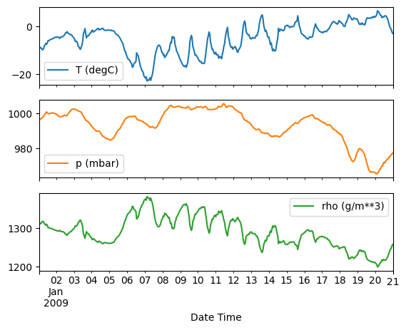
plot_variables(df, date_time)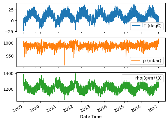
train_df, val_df, test_df, num_features, column_indices = split_data(df)
train_df.shape, val_df.shape, test_df.shape
((49063, 14), (14018, 14), (7010, 14))train_df.head()| p (mbar) | T (degC) | Tpot (K) | Tdew (degC) | rh (%) | VPmax (mbar) | VPact (mbar) | VPdef (mbar) | sh (g/kg) | H2OC (mmol/mol) | rho (g/m**3) | wv (m/s) | max. wv (m/s) | wd (deg) | |
|---|---|---|---|---|---|---|---|---|---|---|---|---|---|---|
| 5 | 996.50 | -8.05 | 265.38 | -8.78 | 94.4 | 3.33 | 3.14 | 0.19 | 1.96 | 3.15 | 1307.86 | 0.21 | 0.63 | 192.7 |
| 11 | 996.62 | -8.88 | 264.54 | -9.77 | 93.2 | 3.12 | 2.90 | 0.21 | 1.81 | 2.91 | 1312.25 | 0.25 | 0.63 | 190.3 |
| 17 | 996.84 | -8.81 | 264.59 | -9.66 | 93.5 | 3.13 | 2.93 | 0.20 | 1.83 | 2.94 | 1312.18 | 0.18 | 0.63 | 167.2 |
| 23 | 996.99 | -9.05 | 264.34 | -10.02 | 92.6 | 3.07 | 2.85 | 0.23 | 1.78 | 2.85 | 1313.61 | 0.10 | 0.38 | 240.0 |
| 29 | 997.46 | -9.63 | 263.72 | -10.65 | 92.2 | 2.94 | 2.71 | 0.23 | 1.69 | 2.71 | 1317.19 | 0.40 | 0.88 | 157.0 |
train_df, val_df, test_df = normalizacion_datos(train_df, val_df, test_df)
train_df.describe()| p (mbar) | T (degC) | Tpot (K) | Tdew (degC) | rh (%) | VPmax (mbar) | VPact (mbar) | VPdef (mbar) | sh (g/kg) | H2OC (mmol/mol) | rho (g/m**3) | wv (m/s) | max. wv (m/s) | wd (deg) | |
|---|---|---|---|---|---|---|---|---|---|---|---|---|---|---|
| count | 4.906300e+04 | 4.906300e+04 | 4.906300e+04 | 4.906300e+04 | 4.906300e+04 | 49063.000000 | 4.906300e+04 | 49063.000000 | 4.906300e+04 | 4.906300e+04 | 4.906300e+04 | 4.906300e+04 | 4.906300e+04 | 4.906300e+04 |
| mean | 2.027515e-16 | -1.946415e-16 | 9.685730e-16 | 1.853728e-17 | -6.719765e-16 | 0.000000 | -2.270817e-16 | 0.000000 | -1.506154e-16 | 1.807385e-16 | -2.321795e-15 | 1.540912e-16 | -1.616219e-16 | -2.178131e-16 |
| std | 1.000000e+00 | 1.000000e+00 | 1.000000e+00 | 1.000000e+00 | 1.000000e+00 | 1.000000 | 1.000000e+00 | 1.000000 | 1.000000e+00 | 1.000000e+00 | 1.000000e+00 | 1.000000e+00 | 1.000000e+00 | 1.000000e+00 |
| min | -9.045695e+00 | -3.682079e+00 | -3.707266e+00 | -4.216645e+00 | -3.746587e+00 | -1.609554 | -2.030996e+00 | -0.829861 | -2.022853e+00 | -2.031986e+00 | -3.846513e+00 | -1.403684e+00 | -1.535423e+00 | -1.977937e+00 |
| 25% | -6.093840e-01 | -7.069026e-01 | -6.939982e-01 | -6.697392e-01 | -6.581569e-01 | -0.750526 | -7.786971e-01 | -0.657581 | -7.762466e-01 | -7.761335e-01 | -7.116941e-01 | -7.390786e-01 | -7.595612e-01 | -6.326198e-01 |
| 50% | 5.467421e-02 | 9.450477e-03 | 1.318575e-02 | 5.168967e-02 | 1.989686e-01 | -0.222892 | -1.561120e-01 | -0.383594 | -1.548152e-01 | -1.540757e-01 | -7.847992e-02 | -2.308512e-01 | -2.250786e-01 | 2.674928e-01 |
| 75% | 6.548575e-01 | 7.200265e-01 | 7.123465e-01 | 7.530390e-01 | 8.150841e-01 | 0.533469 | 6.684569e-01 | 0.268164 | 6.650251e-01 | 6.651626e-01 | 6.442168e-01 | 4.793641e-01 | 5.206108e-01 | 6.932912e-01 |
| max | 2.913378e+00 | 3.066661e+00 | 3.041354e+00 | 2.647686e+00 | 1.455361e+00 | 5.846190 | 4.489514e+00 | 7.842254 | 4.550843e+00 | 4.524268e+00 | 4.310438e+00 | 7.724863e+00 | 8.593884e+00 | 2.131645e+00 |
Creación de ventanas
Ejemplo para un problema que dado las últimas 6 mediciones de temperatura va a predecir la siguiente hora de temperatura.

Ejemplo creación dataset ventanas
# Crear un array de 10 minutos y 3 características (features=2), con valores consecutivos para facilitar el entendimiento
datae = np.arange(10 * 3).reshape(10, 3)

# Crear un DataFrame para mostrar los datos de manera más clara
dfe = pd.DataFrame(datae, columns=['Feature_1', 'Feature_2', 'Target'])
dfe.index.name = 'Minuto'

# Mostrar el DataFrame
dfe| Feature_1 | Feature_2 | Target | |
|---|---|---|---|
| Minuto | |||
| 0 | 0 | 1 | 2 |
| 1 | 3 | 4 | 5 |
| 2 | 6 | 7 | 8 |
| 3 | 9 | 10 | 11 |
| 4 | 12 | 13 | 14 |
| 5 | 15 | 16 | 17 |
| 6 | 18 | 19 | 20 |
| 7 | 21 | 22 | 23 |
| 8 | 24 | 25 | 26 |
| 9 | 27 | 28 | 29 |
# La variable a predecir es la última columna (columna final)
targets = datae[2:, -1]  # Los targets son el valor de la columna final (variable a predecir) desplazados por 2 pasos
targets
array([ 8, 11, 14, 17, 20, 23, 26, 29])# Crear el dataset de series temporales
ds = tf.keras.utils.timeseries_dataset_from_array(
data=datae[:-1], # Todas las filas menos la última, porque no hay target para la última fila
targets=targets, # Los valores a predecir son la columna final de la siguiente fila
sequence_length=2, # Usamos secuencias de 2 minutos
sequence_stride=1, # Stride de 1 para obtener todas las posibles ventanas
shuffle=False, # Barajamos las secuencias
batch_size=2 # Agrupamos en lotes de 2 secuencias
)# Mostrar los primeros 5 lotes de inputs y labels, con un formato mejorado
for batch_num, batch in enumerate(ds.take(5), 1):
inputs, labels = batch
print(f"Batch {batch_num}:")
print(f"Inputs shape: {inputs.shape}")
print("Inputs:")
# Imprimir cada secuencia de inputs con su respectiva etiqueta al final
for i, (input_sequence, label) in enumerate(zip(inputs.numpy(), labels.numpy()), 1):
print(f" Sequence {i}:")
print(f" {input_sequence} -> Target: {label}")
print("\n" + "-"*50 + "\n")Batch 1:
Inputs shape: (2, 2, 3)
Inputs:
Sequence 1:
[[0 1 2]
[3 4 5]] -> Target: 8
Sequence 2:
[[3 4 5]
[6 7 8]] -> Target: 11
--------------------------------------------------
Batch 2:
Inputs shape: (2, 2, 3)
Inputs:
Sequence 1:
[[ 6 7 8]
[ 9 10 11]] -> Target: 14
Sequence 2:
[[ 9 10 11]
[12 13 14]] -> Target: 17
--------------------------------------------------
Batch 3:
Inputs shape: (2, 2, 3)
Inputs:
Sequence 1:
[[12 13 14]
[15 16 17]] -> Target: 20
Sequence 2:
[[15 16 17]
[18 19 20]] -> Target: 23
--------------------------------------------------
Batch 4:
Inputs shape: (2, 2, 3)
Inputs:
Sequence 1:
[[18 19 20]
[21 22 23]] -> Target: 26
Sequence 2:
[[21 22 23]
[24 25 26]] -> Target: 29
--------------------------------------------------
Retomando
MAX_EPOCHS = 20

def compile_and_fit(model, window, patience=2):
  early_stopping = tf.keras.callbacks.EarlyStopping(monitor='val_loss',
                                                    patience=patience,
                                                    mode='min')

  model.compile(loss=tf.keras.losses.MeanSquaredError(),
                optimizer=tf.keras.optimizers.Adam(),
                metrics=[tf.keras.metrics.MeanAbsoluteError()])

  history = model.fit(window.train, epochs=MAX_EPOCHS,
                      validation_data=window.val,
                      callbacks=[early_stopping])
  return history
WIDTH_TEMP = 6
window = WindowGenerator(
input_width=WIDTH_TEMP,
label_width=1,
shift=1,
train_df = train_df,
val_df = val_df,
test_df=test_df,
label_columns=['T (degC)'])
windowTotal window size: 7
Input indices: [0 1 2 3 4 5]
Label indices: [6]
Label column name(s): ['T (degC)']# Stack three slices, the length of the total window.
example_window = tf.stack([np.array(train_df[:window.total_window_size]),
np.array(train_df[100:100+window.total_window_size]),
np.array(train_df[200:200+window.total_window_size])])
example_inputs, example_labels = window.split_window(example_window)
print('All shapes are: (batch, time, features)')
print(f'Window shape: {example_window.shape}')
print(f'Inputs shape: {example_inputs.shape}')
print(f'Labels shape: {example_labels.shape}')All shapes are: (batch, time, features)
Window shape: (3, 7, 14)
Inputs shape: (3, 6, 14)
Labels shape: (3, 1, 1)# graficar los datos en las ventanas
window.plot()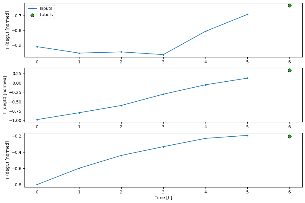
lstm_model = tf.keras.models.Sequential([
    # Shape [batch, time, features] => [batch, time, lstm_units]
    tf.keras.layers.LSTM(32, return_sequences=True),
    # Shape => [batch, time, features]
    tf.keras.layers.Dense(units=1)
])print('Input shape:', window.example[0].shape)
print('Output shape:', lstm_model(window.example[0]).shape)Input shape: (32, 6, 14)
Output shape: (32, 6, 1)history = compile_and_fit(lstm_model, window)
val_performance = {}
performance = {}
val_performance['LSTM'] = lstm_model.evaluate(window.val, return_dict=True)
performance['LSTM'] = lstm_model.evaluate(window.test, verbose=0, return_dict=True)Epoch 1/20 1534/1534 ━━━━━━━━━━━━━━━━━━━━ 14s 8ms/step - loss: 0.1676 - mean_absolute_error: 0.2821 - val_loss: 0.0809 - val_mean_absolute_error: 0.1999 Epoch 2/20 1534/1534 ━━━━━━━━━━━━━━━━━━━━ 12s 8ms/step - loss: 0.0787 - mean_absolute_error: 0.1963 - val_loss: 0.0758 - val_mean_absolute_error: 0.1910 Epoch 3/20 1534/1534 ━━━━━━━━━━━━━━━━━━━━ 12s 8ms/step - loss: 0.0735 - mean_absolute_error: 0.1877 - val_loss: 0.0735 - val_mean_absolute_error: 0.1872 Epoch 4/20 1534/1534 ━━━━━━━━━━━━━━━━━━━━ 18s 6ms/step - loss: 0.0716 - mean_absolute_error: 0.1845 - val_loss: 0.0726 - val_mean_absolute_error: 0.1848 Epoch 5/20 1534/1534 ━━━━━━━━━━━━━━━━━━━━ 11s 7ms/step - loss: 0.0704 - mean_absolute_error: 0.1826 - val_loss: 0.0723 - val_mean_absolute_error: 0.1830 Epoch 6/20 1534/1534 ━━━━━━━━━━━━━━━━━━━━ 20s 7ms/step - loss: 0.0696 - mean_absolute_error: 0.1809 - val_loss: 0.0715 - val_mean_absolute_error: 0.1817 Epoch 7/20 1534/1534 ━━━━━━━━━━━━━━━━━━━━ 20s 7ms/step - loss: 0.0692 - mean_absolute_error: 0.1806 - val_loss: 0.0704 - val_mean_absolute_error: 0.1806 Epoch 8/20 1534/1534 ━━━━━━━━━━━━━━━━━━━━ 20s 7ms/step - loss: 0.0685 - mean_absolute_error: 0.1791 - val_loss: 0.0708 - val_mean_absolute_error: 0.1817 Epoch 9/20 1534/1534 ━━━━━━━━━━━━━━━━━━━━ 23s 8ms/step - loss: 0.0681 - mean_absolute_error: 0.1784 - val_loss: 0.0709 - val_mean_absolute_error: 0.1836 438/438 ━━━━━━━━━━━━━━━━━━━━ 2s 4ms/step - loss: 0.0694 - mean_absolute_error: 0.1819
performance{'LSTM': {'loss': 0.06843273341655731,
'mean_absolute_error': 0.1830073744058609}}val_performance{'LSTM': {'loss': 0.07088509947061539,
'mean_absolute_error': 0.18363438546657562}}